Introduction to Neural Networks

In this post we will give a brief overview of the intution behind neural networks and the math associated with them. Then we will discuss the three stages of training the neural networks:

1. Forward propagation (Forward pass)
2. Backward propagation: Calculation of the loss function
3. Gradient descent: updating the weights and biases

Understanding Their Power

Neural networks are at the forefront of artificial intelligence, possessing the remarkable ability to uncover and model the intricate and nonlinear relationships between inputs and outputs. These advanced computational models excel at generalizing and inferring from data, making them invaluable in handling highly volatile datasets. Beyond their predictive capabilities, neural networks shine in identifying hidden patterns and relationships, enabling them to forecast rare and unusual events with surprising accuracy.

The Intuition Behind Neural Networks

Imagine a vast network of interconnected nodes, each operating in a manner reminiscent of the neurons in our brain. This analogy isn’t just poetic; it’s foundational to understanding how neural networks function.

The Node: A Digital Neuron

At the heart of this network lies the node, a digital counterpart to the human brain’s neurons. Nodes activate in response to significant stimuli, often originating from computational processes. This activation isn’t random; it’s triggered by a weighted sum of inputs from nodes in the previous layer, reflecting a neuron’s response to incoming signals.

Activation: The Essence of Neural Computation

Activation Range: The activation within a node typically falls within one of two ranges: either between -1 and 1 or between 0 and 1. This range is pivotal as it mirrors the biological activity of neurons, which simulates the ‘all-or-nothing’ firing response of neurons in a way that’s conducive to computational modeling.

By mimicking the structure and functionality of the brain’s neural network, artificial neural networks leverage the collective power of these interconnected nodes to process, learn from, and make predictions about complex data, opening up a world of possibilities across various fields.

Neural Network Training Overview: Variables and Terminology

Training a neural network involves adjusting various parameters to minimize the difference between the predicted output and the actual target values. These components include weights, neurons, activation functions, biases, and the inputs and outputs of the system. Below, we delve into each component, shedding light on their purposes, values, and the mathematical notation relevant to their operation.

Neurons (Activation Values)

• Notation: Represented as $a$, neurons are the fundamental processing units of a neural network. The activation value of a neuron is determined by applying an activation function to the weighted sum of inputs from the preceding layer, plus a bias term.
• Value Range: $N \in (-1, 1)$ or $N \in (0, 1)$.
  • Application Considerations: The specific range for neuron outputs is determined by the activation function and the neural network’s task. Selecting the appropriate range is crucial for effective learning and generalization.
    • TBD if we wanna detail more about this! kinda vague on which range to choose right now
  • Addressing Gradient Issues: A well-chosen range helps mitigate the vanishing or exploding gradient problem, facilitating more stable training.

Weights

• Notation: Let $w$ denote the weight associated with a connection between neurons. parameters represent the strength of the connection between neurons across layers. Weights modulate the input signals before summation and application of the activation function.
• Value Range: Unlike neuron activations, weights ($w$) are not restricted to a specific range and may adopt large values to accurately model the relationships between neurons.

Bias

• Notation: Represented by $b$, a bias term allows the activation function to be shifted to left or right to better fit the data.

Activation Functions

• Purpose: Activation functions determine how a neuron’s weighted input is transformed to an output. They introduce non-linearity into the network, enabling it to learn complex patterns. Activation typically map a weighted sum, $z$ to an output in the aforementioned neuron range.

Inputs

• Normalization: Input values must often be normalized to match the activation range of neurons. For instance, an income value for predicting credit class, say $50,000, might be transformed to $1/50,000$ to fit within the neuron’s operating range.
  • Example: Given an input value $x$ and a target range of $N$, normalization can be represented as $N = \frac{x - \text{min}(x)}{\text{max}(x) - \text{min}(x)}$ to scale $x$ into the range $(0, 1)$ or $N = \frac{2(x - \text{min}(x))}{\text{max}(x) - \text{min}(x)} - 1$ for scaling into $(-1, 1)$.

Outputs

• Depending on classification or regression the output layer will look different. For regression we will have 1-d output. For a classificiton problem, we will have a N-d output where N is the number of classes. Think of a problem where we want to predict what number is given as an input(minst dataset), for this we will have 10-D output and expect a 1 in the index of the number we are predicting in the output.

Mathematical Notation and Relationships

• Layer Subscripting: The subscript notation refers to layer numbers, with $L$ denoting the last layer. For example, $a^{(L-1)}$ represents the activations in the penultimate layer, and $a^{(L)}$ for the final layer’s activations.
• Standard Weight Notation: Weights in neural networks are often denoted as $w_{i,j}^{(l)}$, where:
  • $i$ represents the target neuron in the current layer $l$.
  • $j$ represents the source neuron in the previous layer $l-1$.
  • $l$ is the layer number, with the superscript notation $(l)$ indicating that these are the weights leading into layer $l$.

Forward Propagation: The Journey of Input Through the Network

Forward propagation, also known as the forward pass, is the critical process where the input data traverses through the neural network, from the input layer all the way to the output layer. This journey involves a series of linear and nonlinear transformations that gradually refine the data into a prediction. The final output is the prediction made by the network based on its current state (weights and biases). Let’s break down this process and its components for a clearer understanding.

The Process

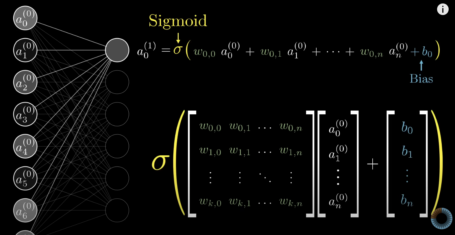
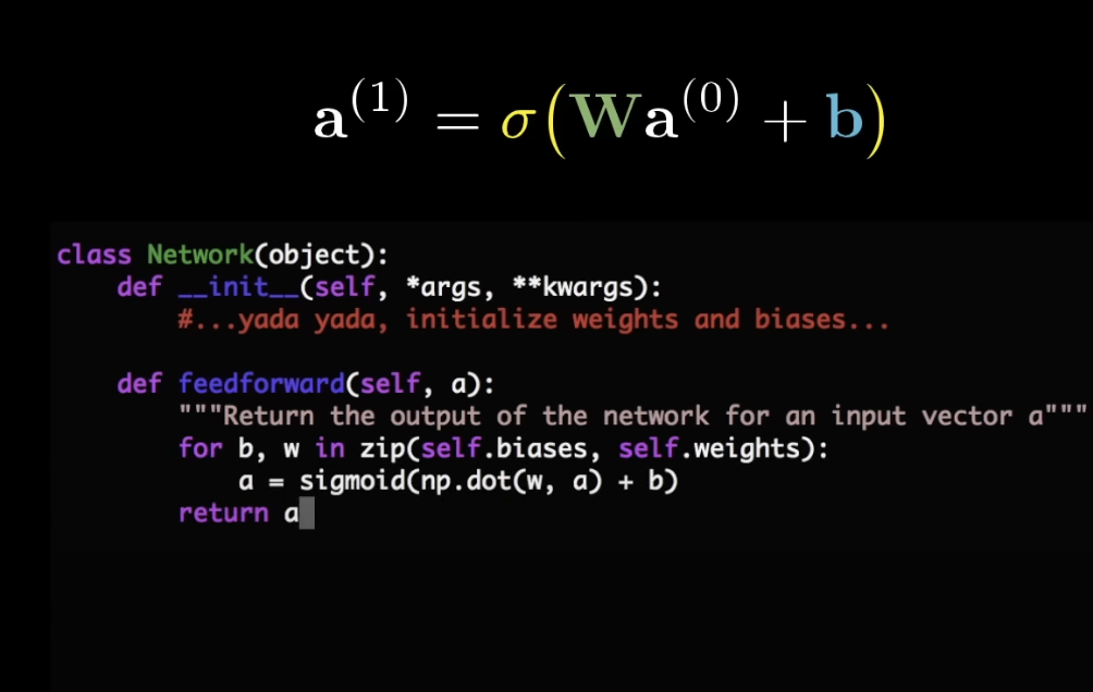
• Linear Transformation: At each layer, the input is transformed linearly using weights ($w$) and biases ($b$). This step can be mathematically represented as $z_{i}^{(l)} = w_{i,j}^{(l)}a_j^{(l-1)} + b_i^{(l)}$, where $a_j^{(l-1)}$ is the activation from the previous layer or the input data for the first layer.
• Nonlinear Activation: Following the linear transformation, a nonlinear activation function is applied to $z_i^{(l)}$, resulting in $a_i^{(l)} = \sigma(z_i^{(l)})$. This activation is then passed on to the next layer as its input.

boils down to: $a^{(1)} = \sigma(\bold{W}a^{(0)}+\bold{b})$ easy to translated to code:

Activation Functions: The Heart of Nonlinearity

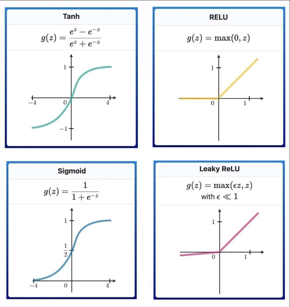
Activation functions introduce nonlinearity into the network, enabling it to learn complex patterns beyond what linear models can capture. These functions are both nonlinear and differentiable, which is crucial for the backpropagation algorithm used during training. Let’s explore some commonly used activation functions:

• Sigmoid: $\sigma(z) = \frac{1}{1 + e^{-z}}$

  • Range: $0$ to $1$
  • Use Case: Ideal for binary classification, providing a clear distinction between two classes.
  • Characteristics: The sigmoid function maps any input to a value between 0 and 1, effectively indicating the positivity of the input.

• ReLU (Rectified Linear Unit): $ReLU(z) = max(0, z)$

  • Range: $0$ to $\infty$
  • Use Case: Commonly used in hidden layers due to its simplicity and efficiency.
  • Characteristics: By zeroing out negative values, ReLU helps with computational efficiency and mitigates the vanishing gradient problem.

• Tanh (Hyperbolic Tangent): $tanh(z) = \frac{e^{z} - e^{-z}}{e^{z} + e^{-z}}$

  • Range: $-1$ to $1$
  • Use Case: Useful when negative outputs are needed for interpretation.
  • Characteristics: Scales the output to between -1 and 1, making it a normalized version of sigmoid for certain applications.

Specialized Activation Function: Softmax

• Softmax: Used in the output layer for multi-class classification, providing a probability distribution across multiple classes.
• Selection Criteria: The choice between Sigmoid and Softmax is dictated by the nature of the task: binary classification (Sigmoid) vs. multi-class classification (Softmax).

Backward Propagation: Computing $-\nabla C$

• do all this for each training example. called stoichastic gradient descent

After the forward pass, the prediction is compared to the actual target value using a loss function, which quantifies the difference between the predicted and true values. Backpropagation is then used to calculate the gradient of the loss function with respect to each weight in the network, moving from the output layer back through the network’s layers. This process relies on the chain rule from calculus to efficiently compute gradients at each layer. done on one training example

The Role of the Loss Function

The journey of learning begins by quantifying the network’s error, achieved through a loss function. The loss function measures the discrepancy between the neural network’s predicted output and the actual target values. Commonly used loss functions include Mean Squared Error (MSE) for regression tasks and Cross-Entropy Loss for classification tasks.

• Mean Squared Error (MSE): $L = \frac{1}{n} \sum (y_i - \hat{y}_i)^2$, where $y_i$ is the actual value and $\hat{y}_i$ is the predicted value for the $i^{th}$ observation.
• Cross-Entropy Loss: For binary classification, $L = -\frac{1}{n} \sum [y_i \log(\hat{y}_i) + (1 - y_i) \log(1 - \hat{y}_i)]$, where $y_i$ is the actual class (0 or 1) and $\hat{y}_i$ is the predicted probability of the class being 1.

Gradient Intuition

• The network computes gradients as vectors pointing towards the steepest loss increase, revealing how small weight changes influence loss. This sensitivity is gauged by the gradient’s magnitude, using calculus’ chain rule to break down complex functions for easier computation.
• Through backpropagation, the network calculates these gradients from the output layer backward, assessing how each weight and bias adjustment affects overall loss.

Backpropagation Calculus

# of parameters in NN with $L$ layers and $N_l$ neurons per layer:

• $W$ can be calculated as: $W = \sum_{l=1}^{L} N_l * N_{l-1}$
• And the total number of biases $B$ is: $B = \sum_{l=1}^{L} N_l$
• The overall total params (weights and biases) is: $T = W + B$

Throughout this walkthrough we will assume the gradient is calcualted every observation. In the next section, we will explore alternative techniques

Lets assume MSE as the error term

$C=\frac{1}{n}\sum_{i=1}^{n}(y_i-a_i^{l})^2$ where $n$ is number of training samples, $y_i$ is actual value and $a_i^{(l)}$ is the predicted value

$a_i^{(L)} = \sigma(z_i^{(L)})$ and $z_i^{(L)} = w_{i,j}^{(L)}a_j^{(L-1)} + b_i^{(L)}$

for any layer term $l$ we can write $a_j^{(l)} = \sum_{k=0}^{n_l}w_{j,k}^{(l)}a_k^{(l-1)}+b_j^{(l)}$

So we can say that the cost function is a function of the weights and biases of the network, thus $\nabla C = \left[ \frac{\partial C}{\partial b_{0}^{(1)}}, \frac{\partial C}{\partial w_{0,0}^{(1)}}, \ldots, \frac{\partial C}{\partial b_{j}^{(l)}}, \frac{\partial C}{\partial w_{j,k}^{(l)}}, \ldots, \frac{\partial C}{\partial b_{n_L}^{(L)}}, \frac{\partial C}{\partial w_{n_L, n_{L-1}}^{(L)}} \right]$

Now we want to solve for each of these partial derivatives. We will start with the weight term and then move to the bias term.

Weight Term

Let’s use the chain rule here to break down a partial derivateiv of a weight w.r.t the cost for observation $i$ and neuron $j$ in layer $l$ as follows:

$\frac{\partial C_i}{\partial w_{j,k}^{(l)}} = \frac{\partial C_i}{\partial a_j^{(l)}} \cdot \frac{\partial a_j^{(l)}}{\partial z_j^{(l)}} \cdot \frac{\partial z_j^{(l)}}{\partial w_{j,k}^{(l)}}$

intuition behind this: Mathematically, this is an application of the multivariate chain rule because $C$ is a function of $a^{(L)}$, which in turn is a function of $z^{(L)}$, which finally is a function of $w^{(L)}$.

some helpful equations:

• $z_j^{(l)} = \sum_k w_{j,k}^{(l)} a_k^{(l-1)} + b_j^{(l)}$

• $a_j^{(l)} = f(z_j^{(l)})$

• $C_i=(y_i-a_i^{L})^2$ for the last layer. understanding how this works in the hidden layers is where backpropagation comes into play

Thus $\frac{\partial C_i}{\partial w_{j,k}^{(L)}} = a_k^{(L-1)} \cdot f'(z_j^{(L)}) \cdot 2(a_j^{(L)}-y_i)$ for the output layer and more generally:

For a weight $w_{j,k}^{(l)}$ in a hidden layer $l$, the gradient of the cost function $C_i$ is:

$\frac{\partial C_i}{\partial w_{j,k}^{(l)}} = a_k^{(l-1)} \cdot f'(z_j^{(l)}) \cdot \left(\sum_{m} w_{m,j}^{(l+1)} \delta_m^{(l+1)}\right)$

where:

• The sum over $m$ accumulates the contribution of neuron $j$ in layer $l$ to the errors of all neurons $m$ in the next layer $(l+1)$, with $\delta_m^{(l+1)}$ being the error of the $m$-th neuron in the next layer, calculated as $f'(z_m^{(l+1)}) \cdot 2(a_m^{(l+1)} - y_i)$ for the output layer or propagated error for other hidden layers.
• $w_{m,j}^{(l+1)}$ are the weights connecting the $j$-th neuron in layer $l$ to the $m$-th neuron in layer $l+1$.

Bias Term

$\frac{\partial C}{\partial b_j^{(l)}} = \frac{\partial z_j^{(l)}}{\partial b_j^{(l)}} \cdot \frac{\partial a_j^{(l)}}{\partial z_j^{(l)}} \cdot \frac{\partial C}{\partial a_j^{(l)}}$

Thus $\frac{\partial C_i}{\partial w_{j,k}^{(L)}} = f'(z_j^{(L)}) \cdot 2(a_j^{(L)}-y_i)$ for the output layer and more generally:

$\frac{\partial C_i}{\partial w_{j,k}^{(l)}} = \cdot f'(z_j^{(l)}) \cdot \left(\sum_{m} w_{m,j}^{(l+1)} \delta_m^{(l+1)}\right)$

Gradient descent

Use Gradient Descent to iteratively update these parameters to minimize the cost function. The algorithm updates the parameters in the opposite direction of the gradient of the cost function with respect to those parameters, gradually moving towards the minimum.

Update Rules

The parameters of the neural network are updated at each step of the Gradient Descent algorithm using the following rules:

• Weights Update Rule: $w_{j,k}^{(l)} := w_{j,k}^{(l)} - \eta \frac{\partial C}{\partial w_{j,k}^{(l)}}$

• Biases Update Rule: $b_j^{(l)} := b_j^{(l)} - \eta \frac{\partial C}{\partial b_j^{(l)}}$

where:

• $\eta$ (eta) is the learning rate, a positive scalar determining the size of the step the algorithm takes at each iteration. The learning rate is a crucial hyperparameter that can affect the convergence of the algorithm: too small, and the algorithm will converge very slowly; too large, and the algorithm might overshoot the minimum or even diverge.

Convergence Criterion

Gradient Descent iterates until a certain convergence criterion is met, such as a small change in the cost function between iterations, a fixed number of iterations, or when the gradient is close to zero, indicating that a minimum (or at least a local minimum) has been reached.

Variants of Gradient Descent

• Stochastic Gradient Descent (SGD): Updates parameters for each training example. It’s faster and can escape local minima better but is noisier.
• Mini-batch Gradient Descent: Updates parameters for small batches of training examples. It balances the speed of SGD and the stability of batch gradient descent.
• Batch Gradient Descent: Updates parameters after computing the gradient on the entire training dataset. It’s stable but can be very slow for large datasets.