We will go through the intuition and math behind the transformer model, as published in the paper Attention is All You Need. The transformer model is a deep learning model that is based on the self-attention mechanism. It is used in natural language processing tasks like machine translation, text summarization, and question-answering systems. It is highly parallelizable and has been shown to outperform traditional RNN-based models on many tasks.

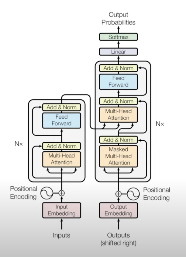
This is the architecure diagram given by the authors in the paper. The model consists of an encoder and a decoder. The encoder is responsible for encoding the input sequence, and the decoder is responsible for generating the output sequence. The encoder and decoder are made up of multiple layers of the same architecture. Each layer has two sub-layers: a multi-head self-attention mechanism and a feed-forward neural network. The output of each sub-layer is passed through a residual connection and a layer normalization operation. The output of the encoder is passed to the decoder, which generates the output sequence.

That was a mouthful, with some unfamilar terms. Let’s break it down

Attention Mechanism

We will start with the attention mechanism. The attention mechanism is a mechanism that allows the model to focus on different parts of the input sequence when generating the output sequence. The attention mechanism is used in the encoder and decoder to capture the dependencies between the input and output sequences.

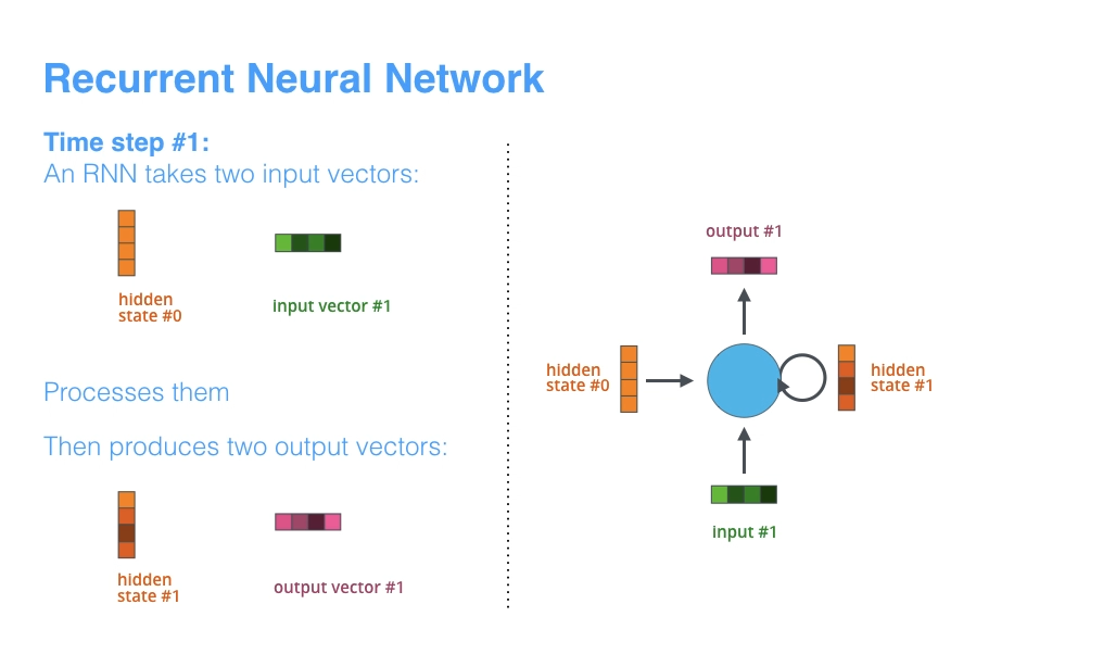
To illustrate the attention mechanism, we will first explore how Seq2Seq Machine Translation model with an encoder and decoder, but they will both be a more familar model, namely an RNN. RNNs always take two inputs: the input sequence and the hidden state. The hidden state is passed from one time step to the next, and it captures the information from the previous time steps. There is also always two outputs: the output sequence and the hidden state.

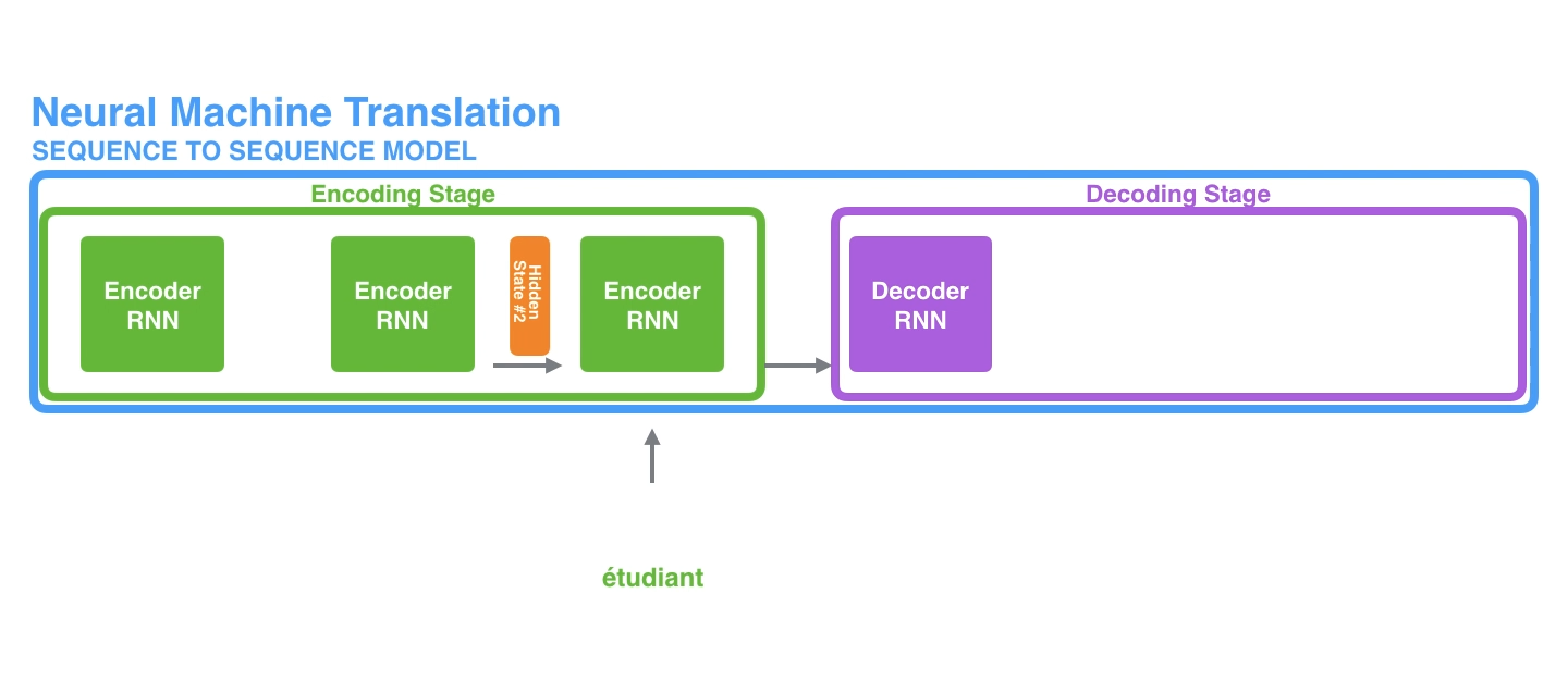
To implore the attention mechanism, we will send all hidden states from the encoder to the decoder. The decoder will then use these hidden states to generate the output sequence.

So now the encoder has completed processing. We are onto the decoder, which has the following structure:

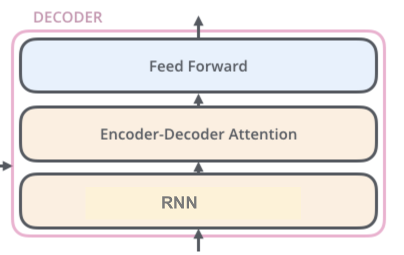
To create the output sequence, the decoder uses the hidden states from the encoder and the previous hidden state as follows:

1. Initial Input: The attention decoder RNN starts with the embedding of a special token (often <sos> or <eos>, depending on the sequence’s direction in the process) and an initial decoder hidden state, which can be the final hidden state produced by the encoder (this varies based on specific model design).
2. RNN Processing: The RNN processes its input (the embedding of the <sos>/<eos> token) along with the initial hidden state, producing an output and a new hidden state vector (let’s call it $h_4$ as an example). Typically, the initial output is ignored, and $h_4$ is used for the attention mechanism.
3. Attention Step: Utilizing the encoder hidden states and the new decoder hidden state $h_4$, the model calculates a context vector $C_4$ for this timestep. This involves scoring each encoder hidden state’s relevance to $h_4$, applying softmax to these scores to get a normalized weight, and then computing the weighted sum of encoder hidden states.
4. Concatenation: The decoder then concatenates $h_4$ and $C_4$ into a single vector. This concatenated vector combines both the current focus of the decoder and the relevant information from the input sequence as highlighted by the attention mechanism.
5. Feedforward Neural Network: This concatenated vector is then passed through a feedforward neural network (often with a softmax layer at the end), which is trained jointly with the rest of the model. This network is responsible for mapping the concatenated vector to a much larger space that represents the probability distribution over the output vocabulary.
6. Output Generation: The output of the feedforward network is interpreted as the next word (or token) in the sequence. This step effectively translates the internal representation (the concatenated vector of $h_4$ and $C_4$) into a specific output element.
7. Iteration for Subsequent Steps: The process repeats for each time step of the sequence generation. For each subsequent step, the decoder uses the previously generated word/token as its new input, updating its hidden state accordingly and recalculating the attention-based context vector for the current focus.

Okay, lets get back to the transformer model. The transformer model uses the self-attention mechanism instead of attention with an RNN. The self-attention mechanism allows for parallel processing of the input sequence, which makes it faster than the RNN.

Self-Attention Mechanism

Self-Attention is a mechanism that allows the model to focus on different parts of the input sequence when generating the output sequence. It bakes the “understanding” of other relevant words into the word the Transformer is currently processing.

The self-attention mechanism is used in the encoder and decoder to capture the dependencies between the input and output sequences.

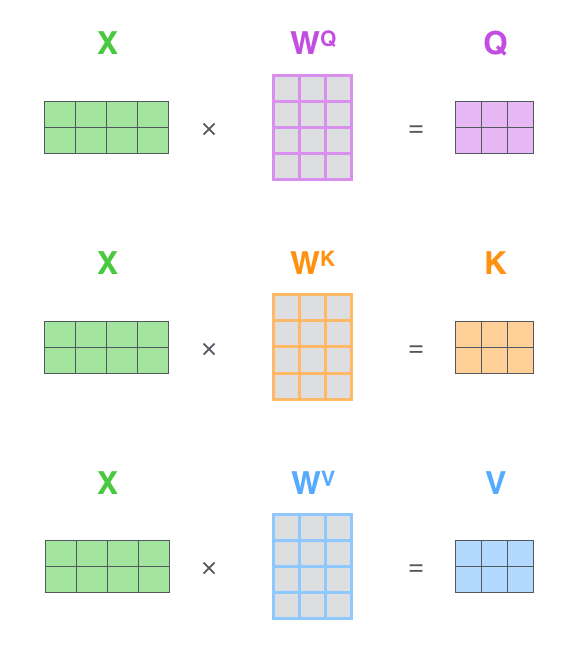
To calcualte self-attention we embed each input token. Then we calculate three vectors for each token: Query, Key, and Value. These vectors are calculated by multiplying the input embeddings by three weight matrices: $W^Q$, $W^K$, $W^V$ which are learned during the training process.

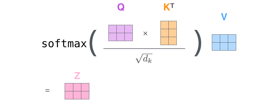
2. Assign a score to each word in relation to the current word by taking the dot product of the Query vector of the current word and the Key vector of the other word. We
3. divide each score by square root of key vector dimension ($\sqrt{d_k}$) - leads to having more stable gradients
4. Apply a softmax function to the scores to get the weights.
5. We then multiply the Value vector of each word by the weights to get the weighted sum.
6. sum the weighted value vectors from step 5. this the $Z$ matrix in the following diagram

Okay, now we can go into the specific names in the transformer model diagram. We will assume a Machine Translation task. Here is a refresher of the model architecture, which we will go thru in order of componets:

General Remarks

There are two components to the Transformer model: the encoder(left) and the decoder(right). The encoder processes the input sequence, and the decoder generates the output sequence. The output of the encoder is passed to the decoder, which ultimately generates the output sequence.

Each compoenent has multiple encoders and decoders respectively($N\times$). These encoders and decoders are identical in structure, but they do not share weights.

Input Embeddings

We start with the input embeddings. We split the input text into tokens and embed each into a learned vector space. The weights of the embedding layer are learned during the training process.

During inference, each token is then mapped to a unique index in a vocabulary, and this index is used to look up the token’s embedding from the embedding layer. These embeddings are essentially dense vector representations that the model learns to associate with each unique token. The collection of all possible token embeddings can be thought of as an embedding matrix, where each row corresponds to the embedding of a token in the vocabulary.

We then add positional encodings to the embeddings to give the model information about the position of the tokens in the sequence. This is similar to what we did above when we pass the hidden states through the encoder RNN model.

Positional Encodings

Positional encodings can be learned during the training process or predefined by a fixed function. A predefined function enhances flexibility at inference time, accommodating sequences longer than those seen during training.

A distinct positional encoding is added to each token embedding. The following code, adapted from a tutorial, demonstrates how to generate these encodings. It interweaves sine and cosine functions to capture each token’s position within the sequence:

# Adapted from https://www.tensorflow.org/tutorials/text/transformer
import numpy as np

def get_angles(pos, i, d_model):
  angle_rates = 1 / np.power(10000, (2 * (i//2)) / np.float32(d_model))
  return pos * angle_rates

def positional_encoding(position, d_model):
  angle_rads = get_angles(np.arange(position)[:, np.newaxis],
                          np.arange(d_model)[np.newaxis, :],
                          d_model)
  
  # Apply sine to even indices in the array (2i)
  angle_rads[:, 0::2] = np.sin(angle_rads[:, 0::2])
  
  # Apply cosine to odd indices in the array (2i+1)
  angle_rads[:, 1::2] = np.cos(angle_rads[:, 1::2])
    
  pos_encoding = angle_rads[np.newaxis, ...]
    
  return pos_encoding

This code successfully generates positional encodings, but let’s delve deeper into its workings. Unlike RNNs, transformers lack an inherent understanding of sequence order. Positional encodings are a means to imbue the model with this spatial awareness, assisting in gradient calculations.

np.newaxis is used to add a new dimension to an array. For instance, if the embedding dimension (d_model) is 512 and the input sequence length is 10, np.arange(position)[:, np.newaxis] results in a shape of (10, 1), and np.arange(d_model)[np.newaxis, :] in a shape of (1, 512).

Examining the angle_rates calculation more closely, (2 * (i//2)) determines the dimension for which we are calculating an angle rate. The alternation between sine and cosine functions for consecutive dimensions ensures they carry non-repeating information, aiding the model’s learning process.

The division by d_model ensures that no exponent exceeds 1, avoiding overly rapid decreases in the sine and cosine waves’ frequencies. This precaution also mitigates potential issues with gradients or numerical stability.

A large base number, such as 10,000, allows for smooth variations between positional encodings, which is crucial for tasks like next-word prediction where relative position offers significant clues. The exponential decay in frequency relative to the dimension index balances the encoding of fine-grained positional information in lower dimensions with more global information in higher dimensions.

Why Use Sine and Cosine?

• Sine and cosine functions embed positional information by their values, leveraging their phase relationship to enable the model, which naturally does not understand sequence order, to infer position.
• The original paper’s authors opted for a mix of sine and cosine functions, finding this approach effective for the model to discern positions through the comparative values and phase relationship of these functions.

This and input embeddings only occur for the first encoder layer. The subsequent layers will receive the output of the previous layer.

Multi-Head Attention - Encoder

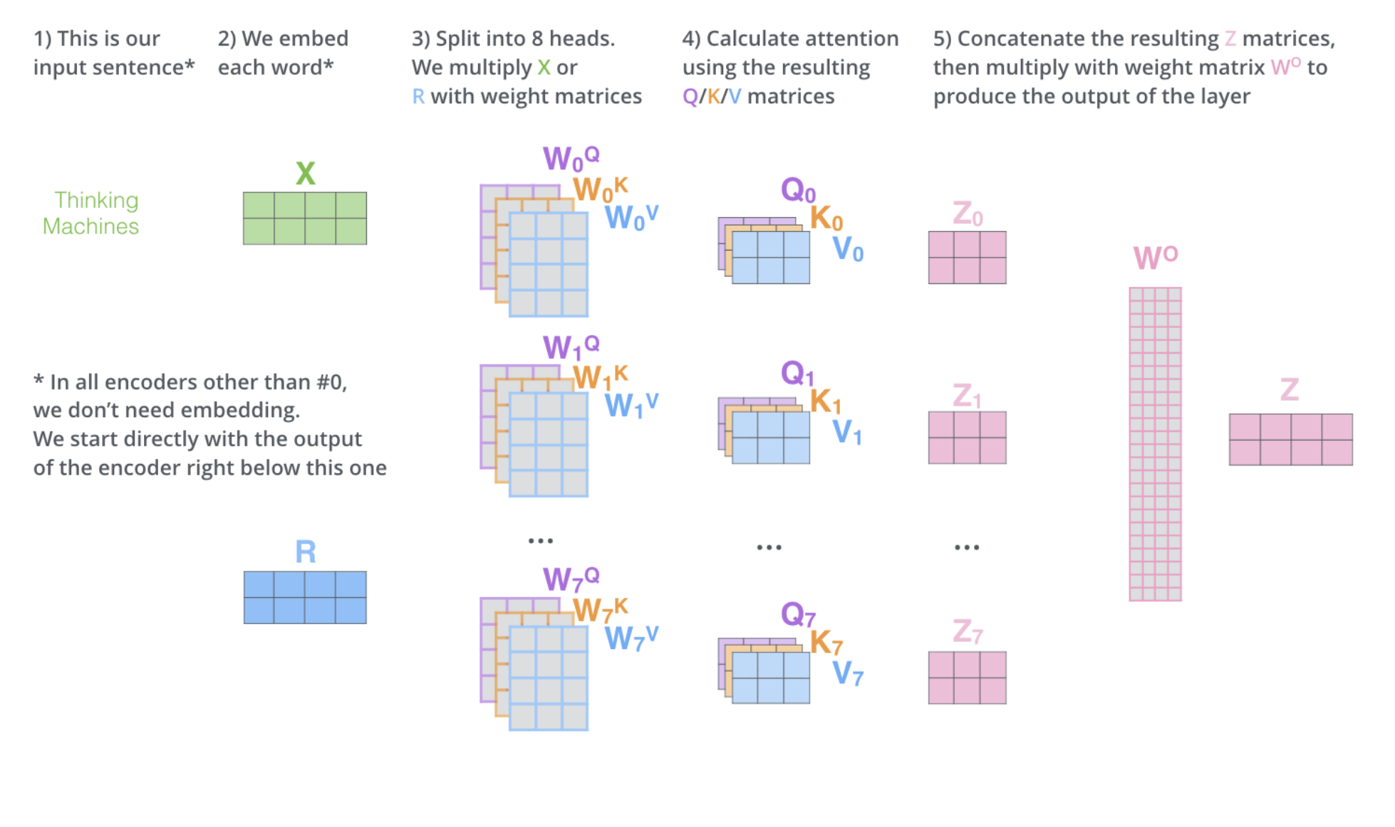
We already went over Self-Attention above. Multi-headed attention means we just do self-attention multiple times with distinct weight matricies. This expands the model’s ability to focus on different positions and gives the attention layer multiple “representation subspaces”. The result is 8 different attention matricies, but the feed forward neural network can only take one. So we concatenate the 8 attention matricies and multiply by a weight matrix(learned during training) to get the final output.

Add & Norm (Multi-Head Attention)

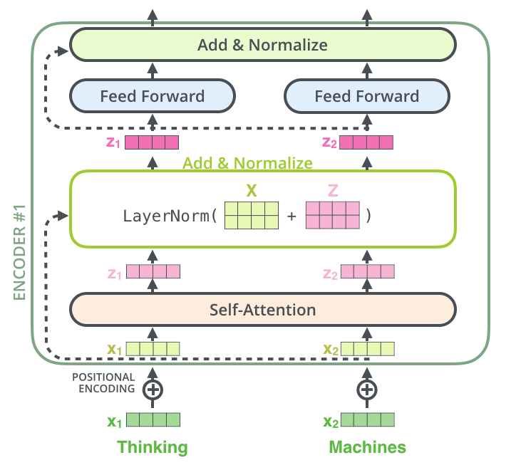
Add: A residual connection around each sub-layer adds the output of the sub-layer to its input, thus “carrying over” the original input. This helps mitigate the vanishing gradient problem by allowing gradients to flow directly through the network. Also helps with residual connections, orignally implemented by ResNet.

Norm: calculates the mean and variance of each vector (here each row of $X + Z$). subtracts the mean from each element and divides by variance so we now we have a standard normal distribution. This normalization helps stabilize the training process and accelerates convergence.

Feed Forward Neural Network - Encoder

We have succesfully baked in relationship with other words. The FFNN transforms the representation of each token independently to allow the model to learn more complex features after integrating information across positions in the self-attention layer.

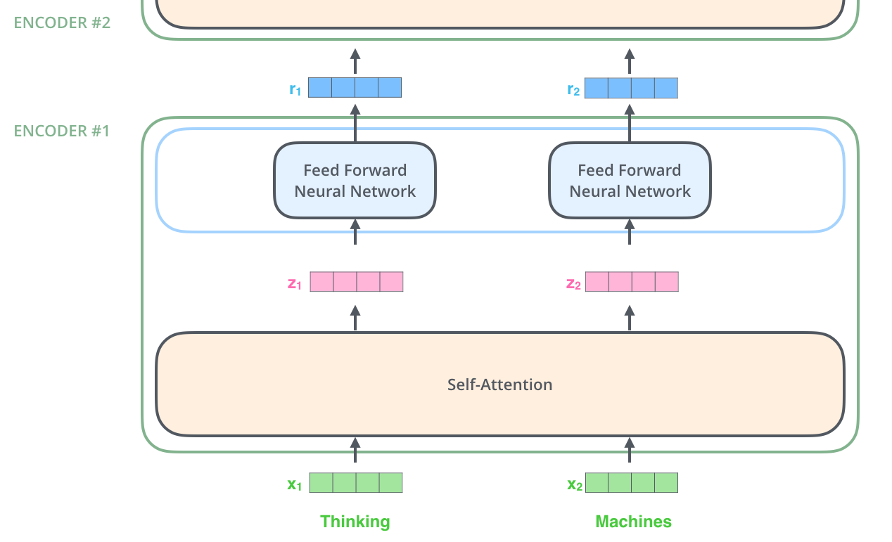
The output of the feed forward neural network is passed through another add & norm layer. The output of this FFNN is then used as the input for the next layer in the encoder or is passed to the decoder if it’s the last encoder layer.

Lets imagine we have gone through all 6 encoders. Encoder outputs a vector for each word. transform into key and value matrix ($K_{encdec}$, $V_{encdec}$) that is used in all decoders of the decoder. They help the decoder focus on correct part of each sequence. We are ready to look at the decoder side.

Outputs (shifted right)

We shift to the right to ensure the decoder is adhering to its autoregressive property(the self-attention layer is only allowed to attend to earlier positions in the output sequence). During training we actually input the correct output sequence and mask future positions by assigning a -inf value to the future positions.

During the first word generation, the decoder is mainly relying on the encoder output. As the decoder generates more words, it starts to rely more on its own output.

Sequential Decoding: Although the entire sequence is fed into the decoder at once, during training, the masked self-attention ensures that each token is predicted based only on the preceding tokens.

Positional Encodings - Decoder

Same as above during training.

During inference, we will have to generate the positional encodings on the fly. We will have to generate the positional encodings after each word generated by the decoder.

Masked Multi-Head Attention - Decoder

The first self-attention layer within each decoder layer is a masked multi-head self-attention layer. This masking ensures that the prediction for a given token can only depend on previously generated tokens, preventing the decoder from “peeking” into the future tokens of the output sequence. The weight matrices for queries ($W_Q$), keys ($W_K$), and values ($W_V$) used in this layer are all learned during training. They are unique to this self-attention layer and are not shared with the encoder or the subsequent encoder-decoder attention layer.

Like in the multi-head attention in the encoder, the input is processed through several parallel attention heads, and the output of each head is concatenated before being passed to the next layer. An additive and normalization step (Add & Norm) follows the attention operation to facilitate learning and stabilize the layer outputs.

Multi-Head Attention - Decoder

This is the second multi-head attention layer in the decoder and is often termed as encoder-decoder attention. Here, the input Q comes from the output of the previous masked self-attention layer in the decoder. The matrices $W_Q$ are unique to each decoder layer and are learned during training, just like the self-attention layer. However, the keys (K) and values (V) weight matricies come from the output of the last layer of the encoder. The weight matrices $W_K$ and $W_V$ associated with the encoder output are also learned during training, but once learned, they are fixed and applied equally across all attention heads in this layer.

The key point here is that while $W_Q$ varies for each attention head within the decoder, $W_K$ and $W_V$ are the same across all heads in this encoder-decoder attention layer. They are also different from the $W_K$ and $W_V$ matrices used in the self-attention layers of the encoder.

After the encoder-decoder attention calculation, the outputs of the different heads are concatenated and then projected down to the original dimensionality with another learned matrix before passing through another additive and normalization step (Add & Norm).

To summarize, both attention mechanisms in the decoder utilize learned weight matrices, but the masked self-attention exclusively focuses on the decoder’s own output up to the current position, while the encoder-decoder attention uses the encoder’s output to inform the generation of the next token in the output sequence.

FFNN, Add & Norm - Decoder

Same as encoder. Expands the dimensionality of the representation of each token independently to allow the model to learn more complex features after integrating information across positions in the self-attention layer.

Linear

The Linear layer is a simple fully connected neural network that projects the vector produced by the stack of decoders, into a much, much larger vector called a logits vector.

Let’s assume that our model knows 10,000 unique English words (our model’s “output vocabulary”) that it’s learned from its training dataset. This would make the logits vector 10,000 cells wide – each cell corresponding to the score of a unique word. That is how we interpret the output of the model followed by the Linear layer.

Softmax

The softmax layer then turns those scores into probabilities (all positive, all add up to 1.0). The cell with the highest probability is chosen, and the word associated with it is produced as the output for this time step. This is called greedy decoding.

Another way to do it would be to hold on to, say, the top two words (say, ‘I’ and ‘a’ for example), then in the next step, run the model twice: once assuming the first output position was the word ‘I’, and another time assuming the first output position was the word ‘a’, and whichever version produced less error considering both positions #1 and #2 is kept. We repeat this for positions #2 and #3…etc. This method is called “beam search”, where in our example, beam_size was two (meaning that at all times, two partial hypotheses (unfinished translations) are kept in memory), and top_beams is also two (meaning we’ll return two translations)

Conclusion

The transformer model is a deep learning model that is based on the self-attention mechanism. It is highly parallelizable and has been shown to outperform traditional RNN-based models on many tasks.

Some transformer based models used in the real world include: BERT, GPT-2, T5, and many more.

Resources:

• https://jalammar.github.io/visualizing-neural-machine-translation-mechanics-of-seq2seq-models-with-attention/
• https://jalammar.github.io/illustrated-transformer/